MitEx#

A core process of many NISQ applications, such as variational algorithms, is the evaluation of the average value of observables for some circuit. This corresponds to measuring the expected value of the bit strings returned by measured qubit shots.

During a typical flow one: defines an ansatz circuit and an observable, produces an appropriate set of measurement circuits, executes all these measurement circuits on a device, calculates their expectation values, and then modifies them by some coefficients, leaving an estimation of the expectation value of the observable.

In its basic capacity, the MitEx.run method will run each of these tasks sequentially, automating the procedure.

from qermit import MitEx
from pytket.extensions.qiskit import AerBackend

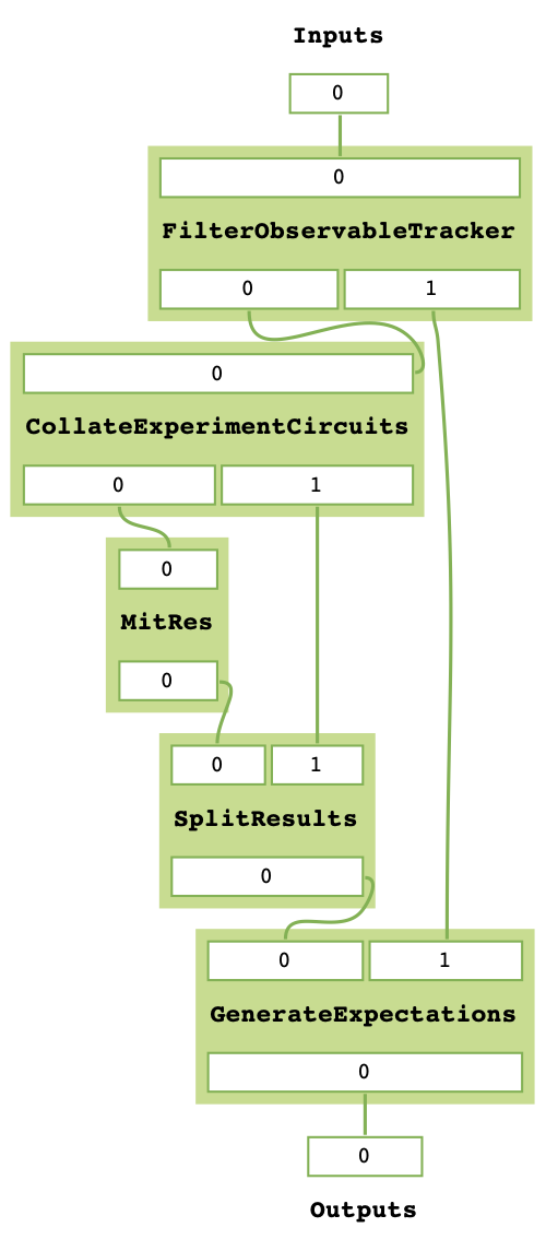
mitex = MitEx(backend = AerBackend())
mitex.get_task_graph()

While the arguments to MitRes will be intuitive to anyone who has used pytket before, the arguments to MitEx may require more consideration (though hopefully sensical to someone who has run an experiment estimating the expectation of an observable before, such as a Variational Quantum Eigensolver experiment).

The MitEx.run method takes List[ObservableExperiment] as an argument, and returns List[QubitPauliOperator]. An ObservableExperiment is a type defined to include the miniumum amount of information necessary to estimate an observable with error-mitigation. ObservableExperiment is a namedtuple with two elements, an AnsatzCircuit and an ObservableTracker.

An AnsatzCircuit Tuple has three elements, a Circuit, the number of device shots to take of Circuit when running on a device, and a SymbolsDict holding a dictionary between symbolic parameters in the Circuit and parameters to subsitute them with. The Circuit object should have no Measure gates, as these will be added during qermit runtime as measurement circuits are produced.

Note that currently qermit can not run variational experiments, but a collection of experiments with different parameters can be passed to MitEx.run at the same time, and the same error-mitigation characteriastions will be used for different experiments where possible.

QubitPauliOperator is a generic data structure from pytket that contains a dictionary from QubitPauliString to a float (for qermit usage). A QubitPauliString is a string of Pauli letters (as used to define Observables to be measured), indexed by a Pytket Qubit.

Finally, an ObservableTracker is an object defined by a QubitPauliOperator that keeps track of both the observable being measured and the measurement circuits required to do so.

from qermit import AnsatzCircuit, SymbolsDict
from pytket.circuit import Circuit, fresh_symbol

sym = fresh_symbol("test")
circuit = Circuit(3,3).X(0).X(1).Rz(sym, 2)
shots = 300
symbols = SymbolsDict.symbols_from_dict({sym: 0.0})
ansatz_circuit = AnsatzCircuit(Circuit=circuit, Shots=shots, SymbolsDict=symbols)

AnsatzCircuit(Circuit=[X q[0]; X q[1]; Rz(test) q[2]; ], Shots=300, SymbolsDict=<SymbolsDict::1>)

from pytket import Qubit
from pytket.pauli import Pauli, QubitPauliString
from pytket.utils import QubitPauliOperator

qubit_pauli_string = QubitPauliString([Qubit(1), Qubit(2)], [Pauli.Z, Pauli.Z])
qubit_pauli_operator = QubitPauliOperator({qubit_pauli_string: 1.0})

print(qubit_pauli_operator)

{(Zq[1], Zq[2]): 1.00000000000000}

from qermit import ObservableTracker

observable_tracker = ObservableTracker(qubit_pauli_operator)

print(observable_tracker)

<ObservableTracker::0MeasurementCircuits>

MitEx will produce and keep track of measurement circuits as it runs, we simply need to construct the object from a QubitPauliOperator as an argument.

from qermit import ObservableExperiment

observable_experiment = ObservableExperiment(AnsatzCircuit = ansatz_circuit, ObservableTracker = observable_tracker)

print(observable_experiment)

ObservableExperiment(AnsatzCircuit=AnsatzCircuit(Circuit=[X q[0]; X q[1]; Rz(test) q[2]; ], Shots=300, SymbolsDict=<SymbolsDict::1>), ObservableTracker=<ObservableTracker::0MeasurementCircuits>)

The MitEx.run method takes List[ObservableExperiment] as an argument, each ObservableExperiment representing a different estimation for a different circuit. For each ObservableExperiment a QubitPauliOperator is returned, giving the expectation value for each QubitPauliString in the operator.

results = mitex.run([observable_experiment])
print(results)

[{(Zq[1], Zq[2]): -1.00000000000000}]

The MitEx constructor has a mitres keyword, which if passed a MitRes object will construct the resulting MitEx from it. This is similar in spirit to the combining of error-mitigation methods discussed in “Combining MitRes methods”.

Error-mitigation with `MitEx`#

As with MitRes, to produce a MitEx object that executes an error-mitigation protocol when MitEx.run is called, additional MitTask objects need to be added to the task graph.

The defining characteristic of a MitEx object is that the first MitTask object in its sorted graph requires a List[ObservableExperiment] object as its sole argument and that the final MitTask object in its sorted graph returns a List[QubitPauliOperator] object. As with MitRes, this is a crucial type constraint required for the combining of error-mitigation methods.

Once more, there are two viable approaches for producing error-mitigation MitEx objects, either extending a MitEx object with new MitTask objects under strict type constraints, or constructing a TaskGraph object with relaxed type constraints on internal tasks and then casting to a MitEx object at completion.

The MitRes section of the manual explains constructing a TaskGraph in great detail and as the process is nearly identical for MitEx we will not explain this again here - if you are interested please refer to that section of the manual. However, we will consider extending a MitEx object with new MitTask objects so as to show the type constraints explicitly.

Extending `MitEx` with `MitTask`#

The MitEx.append and MitEx.prepend methods can be used to extend the MitTask objects the MitEx._task_graph attribute holds.

In some estimation experiments, a priori knowledge about the circuit structure and observable measured can be utilised to discard Shots. This can happen when, for example, some combination of Bits has a value which is known to be impossible. An example of a formal approach to such a method is symmetry verification [Bonet-Monroig2018].

As an example, let’s construct a MitEx object that performs a very basic version of this. While this example will lack physical meaning, it will display how such a method could be written.

from qermit import MitTask
from typing import List, Tuple
from pytket import Bit

def add_ancillas_task_gen(ancillas: List[Tuple[Qubit, Qubit, Bit]]) -> MitTask:
    def task(obj, experiment_wire: List[ObservableExperiment]) -> Tuple[List[ObservableExperiment]]:
        for entry in experiment_wire:
            c = entry.AnsatzCircuit.Circuit
            for tup in ancillas:
                q0 = tup[0]
                q1 = tup[1]
                b = tup[2]

                # check tup is compatible with circuit
                circuit_qubits = entry.AnsatzCircuit.Circuit.qubits
                if q0 not in circuit_qubits:
                    raise ValueError("Circuit has no qubit {}.".format(q0))
                if q1 in circuit_qubits:
                    raise ValueError("Circuit already has ancilla qubit {}.".format(q1))
                if b in entry.AnsatzCircuit.Circuit.bits:
                    raise ValueError("Circuit already had bit {}.".format(b))
                # add new Qubit, add CX between control and ancilla, add Measure
                c.add_qubit(q1)
                c.add_bit(b)
                c.CX(q0, q1)
                c.Measure(q1, b)
        return (experiment_wire,)
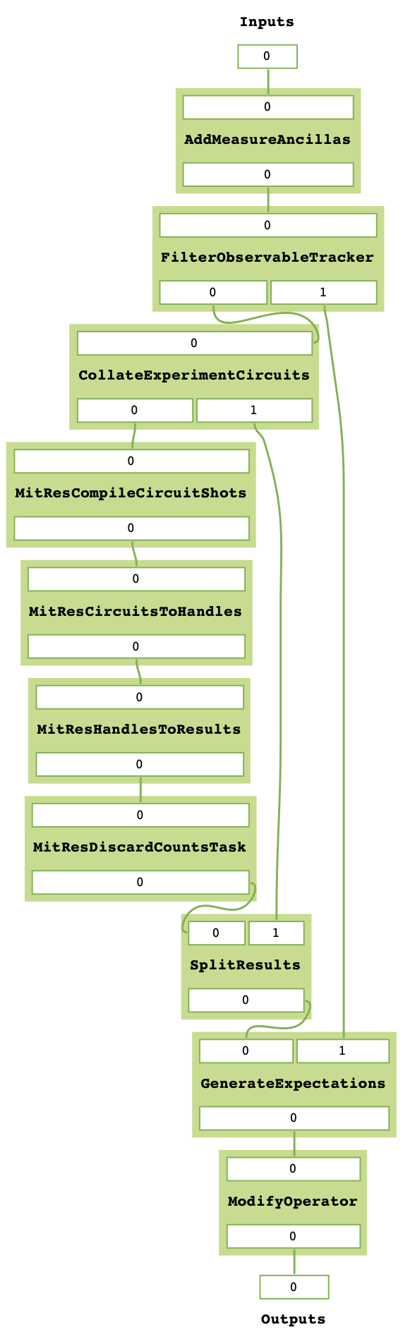
    return MitTask(_label="AddMeasureAncillas", _n_in_wires=1, _n_out_wires=1, _method=task)

The add_ancillas_task_gen function returns a MitTask that modifies the AnsatzCircuit.Circuit to some specification, adding measured ancilla Qubit.

ancillas = [(Qubit(0), Qubit(3), Bit(3))]
ancillas_task = add_ancillas_task_gen(ancillas)
print(ancillas_task)

<MitTask::AddMeasureAncillas>

sim_backend = AerBackend()
mitex_discard = MitEx(backend = sim_backend)
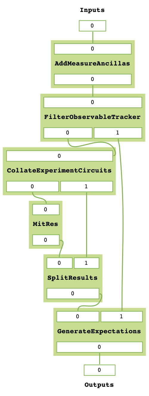
mitex_discard.prepend(ancillas_task)
mitex_discard.get_task_graph()

Clearly this MitTask needs a later corresponding task to process these results. As mentioned earlier, the MitEx constructor accepts a MitRes object from which it constructs its task graph. We can prepare a MitTask that modifies BackendResult given a configuration related to ancillas_task and then prepend it to the MitRes object used for constructing the MitEx object.

from pytket.backends.backendresult import BackendResult
from pytket.utils.outcomearray import OutcomeArray
from typing import Counter

def discard_counts_task_gen(to_discard: List[Tuple[Bit, bool]]) -> MitTask:
    def task(obj, results: List[BackendResult]) -> Tuple[List[BackendResult]]:
        updated_results = []
        for r in results:
            counts = r.get_counts()
            for tup in to_discard:
                bit = tup[0]
                # find entry in counts that corresponds to bit of choice
                count_index = r.c_bits[bit]
                for state in counts:
                    # bit of returned state is banned type
                    if state[count_index] == tup[1]:
                        # remove all counts for banned state
                        counts[state] = 0
            # convert updated Counter to a BackendResult object, add to new results
            counter = Counter(
                {
                    OutcomeArray.from_readouts([key]): val
                    for key, val in counts.items()
                }
            )
            updated_results.append(BackendResult(c_bits = r.c_bits, counts = counter))
        return (updated_results,)
    return MitTask(_label="DiscardCountsTask", _n_in_wires=1, _n_out_wires=1, _method=task)

The discard_counts_task_gen function returns a MitTask object that assigns some counts results in BackendResult to 0 if their Bitstring has some Bit in a specific state.

discard_task = discard_counts_task_gen([(Bit(3), 0)])
print(discard_task)

<MitTask::DiscardCountsTask>

from qermit.taskgraph import backend_compile_circuit_shots_task_gen
from qermit import MitRes

mitres_discard = MitRes(backend = sim_backend)
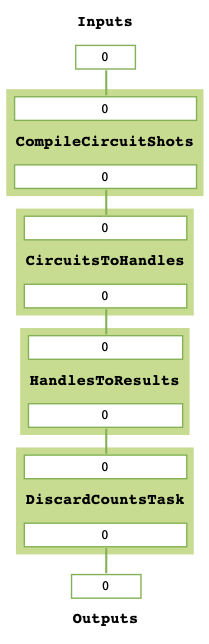
mitres_discard.append(discard_task)
mitres_discard.prepend(backend_compile_circuit_shots_task_gen(sim_backend, optimisation_level = 0))
mitres_discard.get_task_graph()

Lets create a new MitEx object constructed from mitres_discard and then test it.

combined_mitex = MitEx(sim_backend, mitres = mitres_discard)
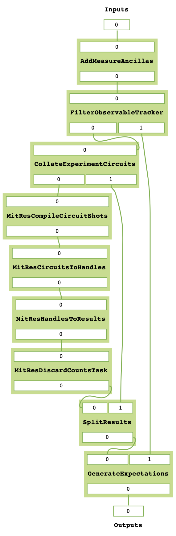
combined_mitex.prepend(add_ancillas_task_gen([(Qubit(0), Qubit(3), Bit(3))]))
combined_mitex.decompose_TaskGraph_nodes()
combined_mitex.get_task_graph()

sym_discard = fresh_symbol("discard_test")
circuit_discard = Circuit(3,3).H(0).X(1).Rz(sym_discard, 2)
shots = 500
symbols = SymbolsDict.symbols_from_dict({sym_discard: 0.0})
ansatz_circuit_discard = AnsatzCircuit(Circuit=circuit_discard.copy(), Shots=shots, SymbolsDict=symbols)

qps = QubitPauliString([Qubit(0), Qubit(1), Qubit(2)], [Pauli.Z, Pauli.Z, Pauli.Z])
qpo_discard = QubitPauliOperator({qps: 1.0})

discard_results = combined_mitex.run([ObservableExperiment(ansatz_circuit_discard, ObservableTracker(qpo_discard))])
print(discard_results)

[{(Zq[0], Zq[1], Zq[2]): 1.00000000000000}]

Without any modification, one would expect the Circuit and measured operator to return either (0,0,1) or (1,0,1) with equal probability, giving a returned expectation value close to 0. However, with the additional ancilla qubit and discarding task, all shots returning (1,0,1) are discarded, leaving an expectation of 1 generated from (0,0,1) shots only.

Considering the MitEx type constraints, we can also append MitTask that receive List[QubitPauliOperator] and return Tuple[List[QubitPauliOperator]].

def modify_operator_task_gen(to_zero: float) -> MitTask:
    def task(obj, results: List[QubitPauliOperator]) -> Tuple[List[QubitPauliOperator]]:
        for operator in results:
            operator_dict = operator._dict
            for string in operator_dict:
                # if absolute of value less than given value, set coefficient to zero
                if abs(operator_dict[string]) < to_zero:
                    operator_dict[string] = 0
        return (results,)
    return MitTask(_label="ModifyOperator", _n_in_wires=1, _n_out_wires=1, _method = task)

As a simple example, this task iterates through every value of every QubitPauliOperator and sets the value to 0 if its value is within some passed range. A more realistic example may modify the values give some characterisation.

combined_mitex.append(modify_operator_task_gen(0.1))
combined_mitex.get_task_graph()

_images/combined_mitex_final_taskgraph.png

ansatz_circuit_discard = AnsatzCircuit(Circuit=circuit_discard.copy(), Shots=shots, SymbolsDict=symbols)

print(combined_mitex.run([ObservableExperiment(ansatz_circuit_discard, ObservableTracker(qpo_discard))]))

[{(Zq[0], Zq[1], Zq[2]): 1.00000000000000}]

Given our discarding tasks, the expectation value returned in this task is always 1.0.

There are several MitEx error-mitigation methods available in qermit; Probabilistic-Error-Cancellation [Temme2016], Zero-Noise-Extrapolation [Giurgica-Tiron2020], Clifford Data Regression with Clifford-Circuit-Learning [Czarnik2020], and Depolarisation-Factor-Supression-For-Nearest-Clifford (an internal method). As with MitRes, each is available via a selection of generator functions.

Probabilistic-Error-Cancellation in `qermit`#

Probabilistic-Error-Cancellation (PEC), introduced in [Temme2016], utilises that it is possible to mitigate for the effect of errors by sampling from a set of erroneous circuits. In particular, a linear combination of the expectation values of an observable measured on a selection of circuit exposed to noise can give an error mitigated expectation value of some fixed primary circuit. Typically this set of circuits is derived from the primary circuit by the addition of certain gates, while the coefficients in the linear combination depend on the noise channel.

If a precise characterisation of the noise model is available, then a means to arrive at both the form and weighting of the set of quantum circuits which perfectly corrects for this model is known [Endo2018] [Temme2016]. Unfortunately, such a characterisation can be very costly to perform if more than a handful of qubits are involved.

To address this, [Strikis2020] introduces a means to learn the appropriate weighting of the noisy circuits. These coefficients are learnt by minimising the error in the final expectation value. As the ideal expectation value of the primary circuit is not known, the training is performed using Clifford circuits which are similar in form to the primary circuit. The expectation of these Clifford circuits can be calculated efficiently using a classical simulator, and so can be compared to the results from noisy runs. It is on this approach that the implementation of PEC in qermit is based.

Generators for Probabilistic-Error-Cancellation MitEx objects are available in the qermit.probabilistic_error_cancellation module.

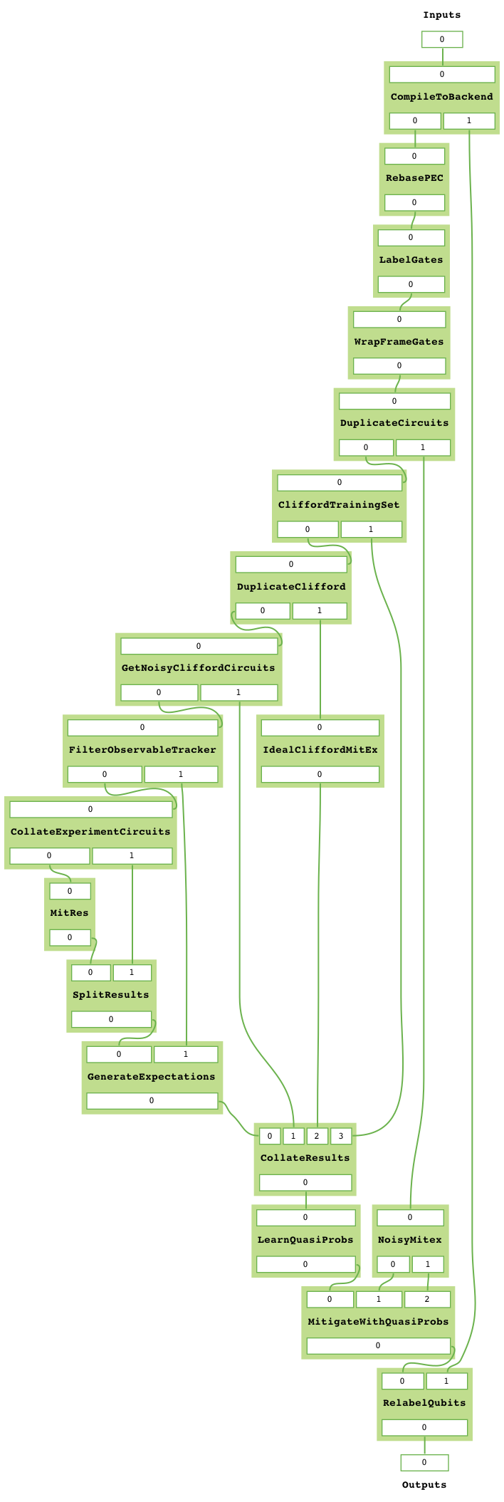
from qermit.probabilistic_error_cancellation import gen_PEC_learning_based_MitEx
from pytket.extensions.qiskit import IBMQEmulatorBackend, AerBackend

noiseless_backend = AerBackend()
lagos_backend = IBMQEmulatorBackend(
  "ibm_lagos",
  hub='',
  group='',
  project='',
)

pec_mitex = gen_PEC_learning_based_MitEx(device_backend = lagos_backend, simulator_backend = noiseless_backend)
pec_mitex.get_task_graph()

Let’s construct a test case with expected value 1.0 and run the error-mitigation MitEx.

from pytket.circuit import Circuit, PauliExpBox, Qubit
from pytket.passes import DecomposeBoxes
from pytket.pauli import Pauli, QubitPauliString
from pytket.utils import QubitPauliOperator

from qermit import ObservableTracker, AnsatzCircuit, SymbolsDict, ObservableExperiment


peb_xyz = PauliExpBox([Pauli.X, Pauli.Y], 0.25)

c = Circuit(2)
c.add_pauliexpbox(peb_xyz, [Qubit(0), Qubit(1)]).Rz(0.2, 0).Rz(0.3, 1)
DecomposeBoxes().apply(c)

qubit_pauli_string = QubitPauliString([Qubit(0), Qubit(1)], [Pauli.Z, Pauli.Z])
ansatz_circuit = AnsatzCircuit(c, 2000, SymbolsDict())

exp = [ObservableExperiment(ansatz_circuit, ObservableTracker(QubitPauliOperator({qubit_pauli_string: 1.0})))]
results = pec_mitex.run(exp)
print(results)

[{(Zq[0], Zq[1]): 1.07030397481665}]

Zero-Noise-Extrapolation in `qermit`#

Zero-Noise-Extrapolation (ZNE), introduced concurrently in [Li2017] and [Temme2016], utilises differing effective device noise levels to perform error correction. In particular, the results of a computation at a variety of noise levels are used to extrapolate to the zero noise limit. This approach acknowledges the difficulty in reducing noise levels, but exploits our ability to increase them. As such, there are two selections to be made when performing ZNE:

The means by which the effective noise levels will be varied.
The method of extrapolation to use to recover the zero noise limit.

Several options exist in both case. Here we will focus on digital ZNE, as discussed in [Giurgica-Tiron2020], as a means to vary the noise level. Digital ZNE is based on the ability to increase noise levels by increasing the number of gates executed. This contrasts with ‘analog’ approaches, which might, for example, alter noise levels by stretching or otherwise changing the pulses acted on superconducting qubits. More specifically we increase the effective noise by performing a folding operation on the circuit, which increases the number of gates without affecting the unitary it implements. At their core these folding methods use that, for a gate \(G\), \(G = G G^{-1} G\), and assume that making this substitution has the affect of tripling the noise.

Extrapolation aims to recover an estimate of the expectation value of some observable, given measured expectation values at the selection of noise levels facilitated by folding. Note that the expectation values and the noise scaling factors are both real numbers. Given these collections of values, and an anzats for the relation between the two, this reduces to a regression problem. There are several ansatz provided by qermit. Each may have its advantages depending on: the device, dominant noise channel, etc.

Generators for Zero-Noise-Extrapolation MitEx objects are available in the qermit.zero_noise_extrapolation module.

from qermit.zero_noise_extrapolation import gen_ZNE_MitEx
from pytket.extensions.qiskit import IBMQEmulatorBackend

zne_mitex = gen_ZNE_MitEx(backend=lagos_backend, noise_scaling_list = [3,5,7])
zne_mitex.get_task_graph()

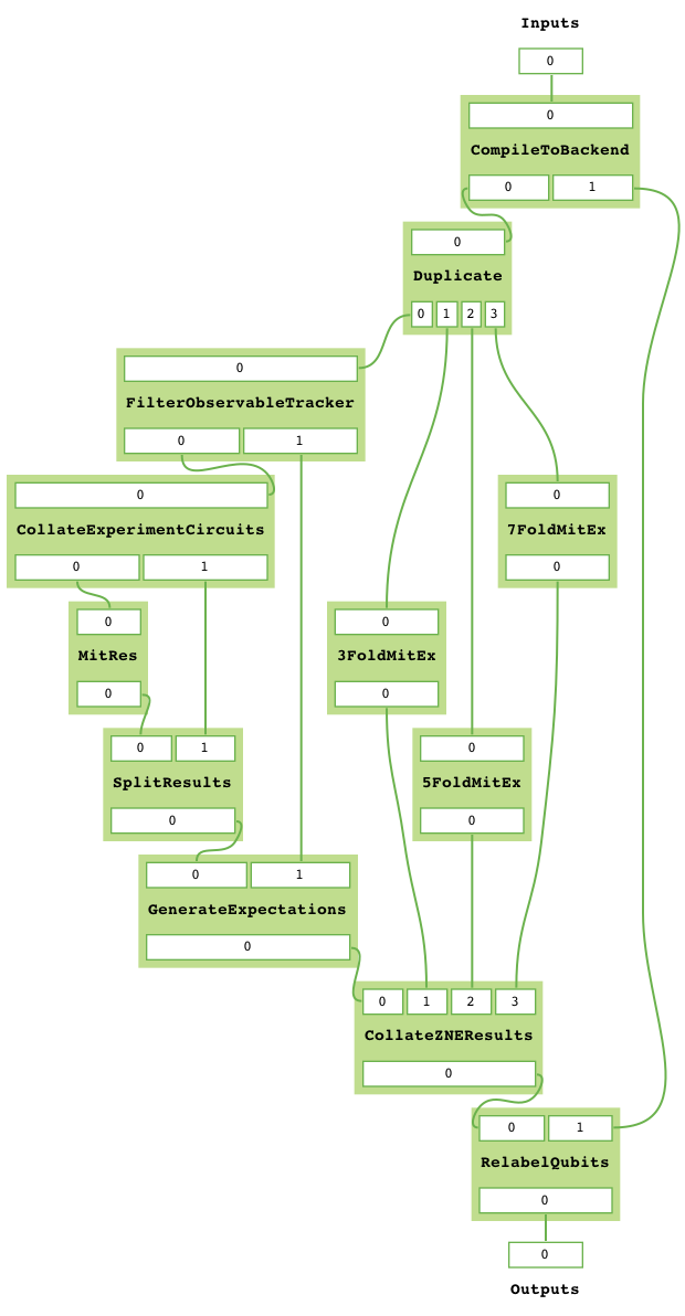
Here the three inputs are: backend, the backend on which the circuits will be run; and noise_scaling_list, a list of integer multiples by which the noise will be scaled. For each noise scaling value a different MitEx object is constructed. Let’s construct a test case with expected value 1.0 and run the error-mitigation MitEx.

from pytket.circuit import Circuit, PauliExpBox, Qubit
from pytket.passes import DecomposeBoxes
from pytket.pauli import Pauli, QubitPauliString
from pytket.utils import QubitPauliOperator

from qermit import ObservableTracker, AnsatzCircuit, SymbolsDict, ObservableExperiment


peb_xyz = PauliExpBox([Pauli.X, Pauli.Y, Pauli.Z], 0.25)

c = Circuit(3)
c.add_pauliexpbox(peb_xyz, [Qubit(0), Qubit(1), Qubit(2)]).Rz(0.2, 0).Rz(0.3, 1).Rz(0.4, 2)
c.add_pauliexpbox(peb_xyz, [Qubit(0), Qubit(1), Qubit(2)]).Rz(0.6, 0).Rz(0.7, 1).Rz(0.8, 2)
c.add_pauliexpbox(peb_xyz, [Qubit(0), Qubit(1), Qubit(2)]).Rz(0.9, 0).Rz(0.1, 1).Rz(0.2, 2)
c.add_pauliexpbox(peb_xyz, [Qubit(0), Qubit(1), Qubit(2)])
DecomposeBoxes().apply(c)

qubit_pauli_string = QubitPauliString(
    [Qubit(0), Qubit(1), Qubit(2)], [Pauli.Z, Pauli.Z, Pauli.Z]
)
ansatz_circuit = AnsatzCircuit(c, 2000, SymbolsDict())

exp = [ObservableExperiment(ansatz_circuit, ObservableTracker(QubitPauliOperator({qubit_pauli_string: 1.0})))]
results = zne_mitex.run(exp)
print(results)

[{(Zq[0], Zq[1], Zq[2]): 0.882900000000000}]

There are many customisation options available when using the zero-noise-extrapolation MitEx generator in qermit, all can be seen via the documentation. The type of folding used for creating digitally noisier circuits can be specified via the _folding_type keyword argument. This expects a Folding object, which default has support for gate folding and circuit folding. The fit used to extrapolate results can be specified via the _fit_type keyword argument. This expects a Fit object, which default has support for a variety of fits.

Clifford-Circuit-Learning and Clifford-Data-Regression in `qermit`#

Correcting device noise typically requires some characterisation of what the noise is, while characterising noise typically requires an understanding of what data would look like without noise.

Clifford-Circuit-Learning uses quantum circuits composed primarily of Clifford gates to characterise and correct for device noise. As such circuits can be efficiently simulated classically this approach has viable scalability.

Given some experiment circuit to run on some device, a set of state circuits are generated for characterisation. Each state circuit is constructed such that it is structurally similar to the experiment circuit, but near Clifford so that it retains the feature of being efficiently simluated classically. In this method, such near Clifford circuits are generated by substituting non-Clifford gates in the experiment Circuit with randomly sampled Clifford gates from a biased distribution.

For each state circuit the ideal expectation value is calculated with a simulator for the desired observable, while the noisy expectation value is calculated by running the circuit on the target device. These results are then used to construct a model for the noise free value of the observable for states in the vicinity of the state the experiment circuit produces. The original experiment circuit is then run on the device and its observable estimate corrected by the model.

In this sense, “Clifford-Circuit-Learning” refers to the general noise characterisation approach defined by efficiently simulated classically Clifford circuits and “Clifford-Data-Regression” refers to the noise correction technique used here.

Generators for Clifford-Data-Regression MitEx objects are available in the qermit.clifford_noise_characterisation module.

from qermit.clifford_noise_characterisation import gen_CDR_MitEx
from pytket.extensions.qiskit import AerBackend, IBMQBackend


noisy_backend = IBMQBackend(
  "ibm_lagos",
  hub='',
  group='',
  project='',
)
noiseless_backend = AerBackend()

cdr_mitex = gen_CDR_MitEx(device_backend = noisy_backend,
                      simulator_backend = noiseless_backend,
                      n_non_cliffords = 2,
                      n_pairs = 2,
                      total_state_circuits = 50)
cdr_mitex.get_task_graph()

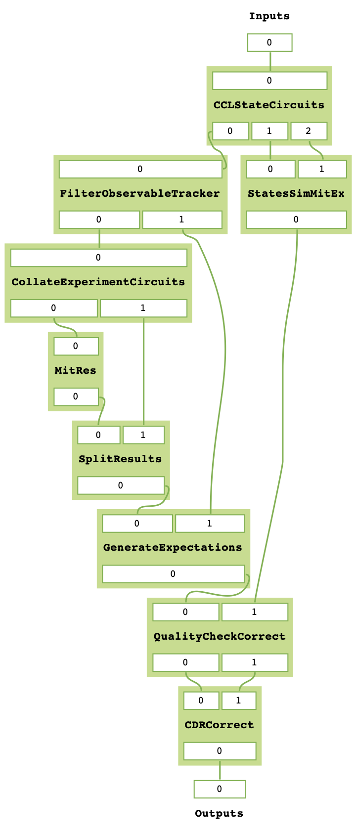
We have avoided decomposing all graph nodes before viewing in this case as there are many nodes required to complete this method (run cdr_mitex.decompose_TaskGraph_nodes() before viewing if interested).

The device_backend argument defines the Backend all noisy state circuit results and the actual experiment results are retrieved and calculated from. The simulator_backend argument defines the Backend all noiseless state circuit results and retrieved and calculated from. The n_non_cliffords arguments defines the number of non-Clifford gates in the produced state circuits for characterisation. In this construction, state circuits are generated via a Markov Chain Monte Carlo technique by making small modifications to other state circuits - the n_pairs argument defines the number of non-Clifford state circuit gates converted to Clifford and vice versa (essentially the ‘distance’ between generated state circuits). The total_state_circuits argument defines the total number of state circuits constructed for characterisation.

These parameters give a large space for optimising the performance of the given method. Furthermore, some keyword arguments allow even more customisation.

The model keyword argument defines the model produced by the characterisation data and expects a _BaseExCorrectModel object. It is by default set to model a linear relationship between noisy and noiseless expectation values, but the _PolyCDRCorect class can be used to define other relationships.

In [Czarnik2020], a Metropolis-Hastings rule is used to accept or reject state circuits from the characterisation data. The likelihood function used in this rule can be defined with the LikelihoodFunction keyword argument, which expects a LikelihoodFunction object. The relationship between performance and choice of LikelihoodFunction is expected to be closely linked to the Circuits run, and so by default the likelihood function is set to accept all results. Be aware that as qermit does not support loops currently, this process is only run after device execution and so if any state circuits are not accepted, no replacement will be found and so the total number of circuits used in characteriastion will be fewer than as originally specified.

Lets test with a basic example with expected result 1.0.

from pytket.circuit import Circuit, PauliExpBox, Qubit
from pytket.passes import DecomposeBoxes
from pytket.pauli import Pauli

peb_xyz = PauliExpBox([Pauli.X, Pauli.Y, Pauli.Z], 0.25)

c = Circuit(3,3)
c.add_pauliexpbox(peb_xyz, [Qubit(0), Qubit(1), Qubit(2)]).Rz(0.2, 0).Rz(0.3, 1).Rz(0.4, 2)
c.add_pauliexpbox(peb_xyz, [Qubit(0), Qubit(1), Qubit(2)]).Rz(0.6, 0).Rz(0.7, 1).Rz(0.8, 2)
c.add_pauliexpbox(peb_xyz, [Qubit(0), Qubit(1), Qubit(2)]).Rz(0.9, 0).Rz(0.1, 1).Rz(0.2, 2)
c.add_pauliexpbox(peb_xyz, [Qubit(0), Qubit(1), Qubit(2)])
DecomposeBoxes().apply(c)

from pytket import Qubit
from pytket.pauli import QubitPauliString, Pauli  # type: ignore
from pytket.utils import QubitPauliOperator
from qermit import ObservableTracker, AnsatzCircuit, SymbolsDict, ObservableExperiment

qubit_pauli_string = QubitPauliString(
    [Qubit(0), Qubit(1), Qubit(2)], [Pauli.Z, Pauli.Z, Pauli.Z]
)
ansatz_circuit = AnsatzCircuit(c, 2000, SymbolsDict())

exp = [ObservableExperiment(ansatz_circuit, ObservableTracker(QubitPauliOperator({qubit_pauli_string: 1.0})))]
cdr_results = cdr_mitex.run(exp)
print(cdr_results)

[{(Zq[0], Zq[1], Zq[2]): 0.822882253534080}]

For comparison we can run the same experiment without error-mitigation.

from qermit import MitEx
mitex = MitEx(noisy_backend)
exp = [ObservableExperiment(ansatz_circuit, ObservableTracker(QubitPauliOperator({qubit_pauli_string: 1.0})))]
results = mitex.run(exp)
print(results)

[{(Zq[0], Zq[1], Zq[2]): 0.729000000000000}]

For the basic example constructed, fairly small 2000 shots and the ibm_lagos device available through IBMQ, we see that the error-mitigated expectation value is closer to the expected value 1.0 than without error-mitigation.

For combining schemes, the StatesSimulatorMitex keyword argument defines the MitEx object for noiseless simluation of all state circuits, the StatesDeviceMitex keyword argument defines the MitEx object for device executions of all state circuits, and the ExperimentMitex object defines the MitEx object all experiment circuits are executed on.

Depolarisation-Factor-Supression-For-Nearest-Clifford in `qermit`#

This method estimates the averaged incoherent noise component affecting the entire circuit structure and reduces its effect on computing expectation values. The main advantage of DFSC is that it does not require significant quantum resource overhead (no additional ancillas and no increased depth) and relies on efficient classical processing. This error-mitigation technique trades-off a finer-grained noise characterisation for scalability (i.e reduced computational resources).

The effect of an incoherent Pauli noise channel when computing expectation values of Pauli operators for a target state is to scale the exact expected value by a factor that depends on the i) noise channel and ii) Pauli observable.

DFSC estimates this factor by assuming that a Clifford circuit derived from the structure of the target quantum circuit will incur similar levels of incoherent noise. This factor results from quantum hardware evaluation of the Pauli observable’s expected value with respect to a state produced by the Clifford circuit acting on a positive eigenstate of a forwarded Pauli operator given by the adjoint action of the Clifford unitary on the target Pauli observable.

The freedom in the choice of eigenstate can be used to extend the present method to allow finer error mitigation at the expense of increased computational resources.

The DFSC method will be most useful when the accumulation of errors through a circuit incurs a loss of purity in the state preparation and incoherent errors dominate. It may be used, for example, in a variational algorithm to adaptively account for these types of errors within the optimisation loop using minimal additional quantum compute time.

Generators for Depolarisation-Factor-Supression-For-Nearest-Clifford MitEx objects are available in the qermit.clifford_noise_characterisation module.

from qermit.clifford_noise_characterisation import gen_DFSC_MitEx
from pytket.extensions.qiskit import IBMQBackend

lagos_backend = IBMQEmulatorBackend(
  "ibm_lagos",
  hub='',
  group='',
  project='',
)
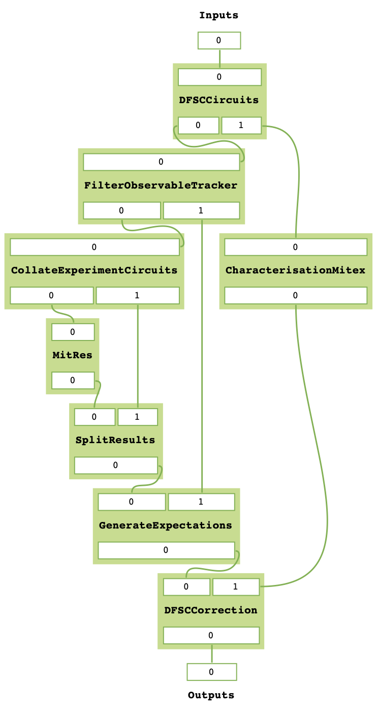
dfsc_mitex = gen_DFSC_MitEx(lagos_backend)
dfsc_mitex.get_task_graph()

The DFSC MitEx expects all non-Clifford gates to be parameterised via the SymbolsDict. Once again, we construct an example that with expected value 1.0.

from pytket.circuit import Circuit, PauliExpBox, Qubit, fresh_symbol
from pytket.passes import DecomposeBoxes
from pytket.pauli import Pauli, QubitPauliString
from pytket.utils import QubitPauliOperator

from qermit import ObservableTracker, AnsatzCircuit, SymbolsDict, ObservableExperiment

sym = fresh_symbol("test")
peb_xyz = PauliExpBox([Pauli.X, Pauli.Y, Pauli.Z], sym)

c = Circuit(3,3)
c.add_pauliexpbox(peb_xyz, [Qubit(0), Qubit(1), Qubit(2)]).Z(0).Z(1).Z(2)
c.add_pauliexpbox(peb_xyz, [Qubit(0), Qubit(1), Qubit(2)]).Z(0).Z(1).Z(2)
c.add_pauliexpbox(peb_xyz, [Qubit(0), Qubit(1), Qubit(2)]).Z(0).Z(1).Z(2)
c.add_pauliexpbox(peb_xyz, [Qubit(0), Qubit(1), Qubit(2)])
DecomposeBoxes().apply(c)


qubit_pauli_string = QubitPauliString(
        [Qubit(0), Qubit(1), Qubit(2)], [Pauli.Z, Pauli.Z, Pauli.Z]
    )
ansatz_circuit = AnsatzCircuit(c, 2000, SymbolsDict.symbols_from_dict({sym: 0.25}))

exp = [ObservableExperiment(ansatz_circuit, ObservableTracker(QubitPauliOperator({qubit_pauli_string: 1.0})))]
dfsc_results = dfsc_mitex.run(exp)
print(dfsc_results)

[{(Zq[0], Zq[1], Zq[2]): 0.848898216159496}]

The MitEx object returned by gen_DFSC_MitEx has both a characterisation and experiment stage. The MitEx characterisation is completed with can be specified with the CharacterisationMitex keyword argument. The MitEx the experiment is completed with can be specified with the ExperimentMitex keyword argument.

[Bonet-Monroig2018]

Bonet-Monroig, X., Sagastizabal, R., Singh, M., O’Brien, T.E., 2018. Low-cost error mitigation by symmetry verification. Phys. Rev. A 98, 062339 (2018).

[Temme2016] (1,2,3,4)

Temme, K., Bravyi, S., Gambetta, J.M., 2016. error mitigation for short-depth quantum circuits. Phys. Rev. Lett. 119, 180509 (2017).

[Giurgica-Tiron2020] (1,2)

Giurgica-Tiron, T., Hindy, Y., LaRose, Ryan., Mari, A., Zeng, W.J., 2020, Digital zero noise extrapolation for quantum error mitigation. 2020 IEEE International Conference on Quantum Computing and Engineering (QCE), Denver, CO, USA, 2020.

[Czarnik2020] (1,2)

Czarnik, P., Arrasmith, A., Coles, P.J., Cincio, L., 2020. error mitigation with Clifford quantum-circuit data. arXiv:2005.10189.

[Li2017]

Li, Y., & Benjamin, S. C. (2017). Efficient variational quantum simulator incorporating active error minimization. Physical Review X, 7(2), 021050.

[Endo2018]

Endo, S., Benjamin, S. C., & Li, Y. (2018). Practical quantum error mitigation for near-future applications. Physical Review X, 8(3), 031027.

[Strikis2020]

Strikis, A., Qin, D., Chen, Y., Benjamin, S. C., & Li, Y. (2020). Learning-based quantum error mitigation. arXiv preprint arXiv:2005.07601.

MitEx

Contents

MitEx#

Error-mitigation with MitEx#

Extending MitEx with MitTask#

Probabilistic-Error-Cancellation in qermit#

Zero-Noise-Extrapolation in qermit#