Training: Quantum case

In this tutorial we will train a lambeq model to solve the relative pronoun classification task presented in [Lea2021]. The goal is to predict whether a noun phrase contains a subject-based or an object-based relative clause. The entries of this dataset are extracted from the RelPron dataset [Rea2016].

We will use an IQPAnsatz to convert string diagrams into quantum circuits. The pipeline uses tket as a backend.

If you have already gone through the classical training tutorial, you will see that there are only minor differences for the quantum case.

Download code

Preparation

We start with importing NumPy and specifying some training hyperparameters.

import os
import warnings

warnings.filterwarnings('ignore')
os.environ['TOKENIZERS_PARALLELISM'] = 'true'

Note

We disable warnings to filter out issues with the tqdm package used in jupyter notebooks. Furthermore, we have to specify whether we want to use parallel computation for the tokenizer used by the BobcatParser. None of the above impairs the performance of the code.

import numpy as np

BATCH_SIZE = 10
EPOCHS = 100
SEED = 2

Input data

Let’s read the data and print some example sentences.

def read_data(filename):
    labels, sentences = [], []
    with open(filename) as f:
        for line in f:
            t = int(line[0])
            labels.append([t, 1-t])
            sentences.append(line[1:].strip())
    return labels, sentences


train_labels, train_data = read_data('../examples/datasets/rp_train_data.txt')
val_labels, val_data = read_data('../examples/datasets/rp_test_data.txt')

train_data[:5]

['organization that church establish .',
 'organization that team join .',
 'organization that company sell .',
 'organization that soldier serve .',
 'organization that sailor join .']

Targets are represented as 2-dimensional arrays:

train_labels[:5]

[[1, 0], [1, 0], [1, 0], [1, 0], [1, 0]]

Creating and parameterising diagrams

The first step is to convert sentences into string diagrams.

Note

We know that the specific dataset only consists of noun phrases, hence, we reduce potential parsing errors by restricting the parser to only return parse trees with the root categories N (noun) and NP (noun phrase).

from lambeq import BobcatParser

parser = BobcatParser(root_cats=('NP', 'N'), verbose='text')

raw_train_diagrams = parser.sentences2diagrams(train_data, suppress_exceptions=True)
raw_val_diagrams = parser.sentences2diagrams(val_data, suppress_exceptions=True)

Tagging sentences.
Parsing tagged sentences.
Turning parse trees to diagrams.
Tagging sentences.
Parsing tagged sentences.
Turning parse trees to diagrams.

Filter and simplify diagrams

We simplify the diagrams by calling normal_form() and filter out any diagrams that could not be parsed.

train_diagrams = [
    diagram.normal_form()
    for diagram in raw_train_diagrams if diagram is not None
]
val_diagrams = [
    diagram.normal_form()
    for diagram in raw_val_diagrams if diagram is not None
]

train_labels = [
    label for (diagram, label)
    in zip(raw_train_diagrams, train_labels)
    if diagram is not None]
val_labels = [
    label for (diagram, label)
    in zip(raw_val_diagrams, val_labels)
    if diagram is not None
]

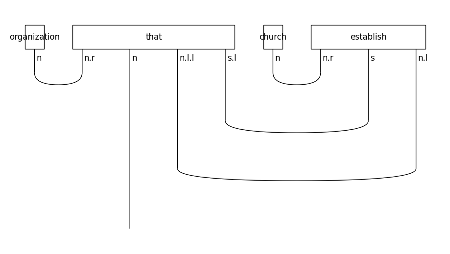
Let’s see the form of the diagram for a relative clause on the subject of a sentence:

train_diagrams[0].draw(figsize=(9, 5), fontsize=12)

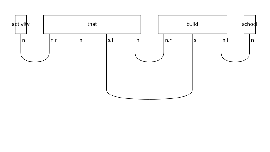
In object-based relative clauses the noun that follows the relative pronoun is the object of the sentence:

train_diagrams[-1].draw(figsize=(9, 5), fontsize=12)

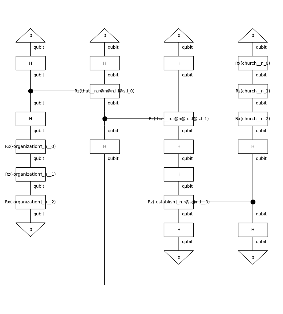
Create circuits

In order to run the experiments on a quantum computer, we need to apply to string diagrams a quantum ansatz. For this experiment, we will use an IQPAnsatz, where noun wires (n) are represented by a one-qubit system, and sentence wires (s) are discarded (since we deal with noun phrases).

from lambeq import AtomicType, IQPAnsatz, RemoveCupsRewriter

ansatz = IQPAnsatz({AtomicType.NOUN: 1, AtomicType.SENTENCE: 0},
                   n_layers=1, n_single_qubit_params=3)
remove_cups = RemoveCupsRewriter()

train_circuits = [ansatz(remove_cups(diagram)) for diagram in train_diagrams]
val_circuits =  [ansatz(remove_cups(diagram))  for diagram in val_diagrams]

train_circuits[0].draw(figsize=(9, 10))

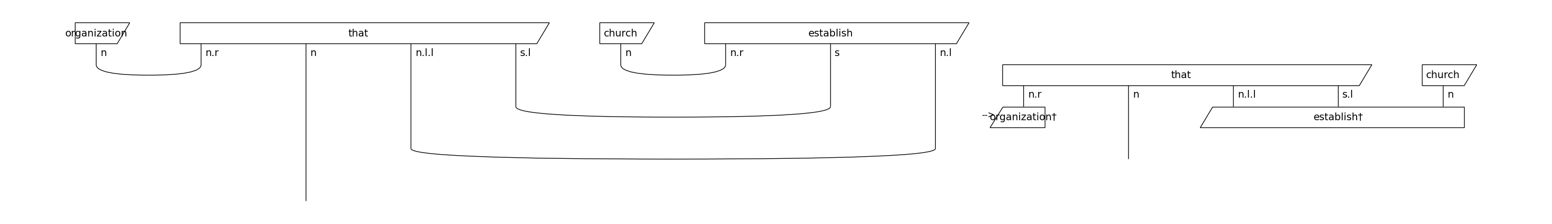
Note that we remove the cups before parameterising the diagrams. By doing so, we reduce the number of post-selections, which makes the model computationally more efficient. The effect of cups removal on a string diagram is demonstrated below:

from lambeq.backend import draw_equation

original_diagram = train_diagrams[0]
removed_cups_diagram = remove_cups(original_diagram)

draw_equation(original_diagram, removed_cups_diagram, symbol='-->', figsize=(30, 6), asymmetry=0.3, fontsize=14)

Training

Instantiate the model

We will use a TketModel, which we initialise by passing all diagrams to the class method TketModel.from_diagrams(). The TketModel needs a backend configuration dictionary passed as a keyword argument to the initialisation method. This dictionary must contain entries for backend, compilation and shots. The backend is provided by pytket-extensions. In this example, we use Qiskit‘s AerBackend with 8192 shots.

from pytket.extensions.qiskit import AerBackend
from lambeq import TketModel

all_circuits = train_circuits + val_circuits

backend = AerBackend()
backend_config = {
    'backend': backend,
    'compilation': backend.default_compilation_pass(2),
    'shots': 8192
}

model = TketModel.from_diagrams(all_circuits, backend_config=backend_config)

Note

The model can also be instantiated by calling TketModel.from_checkpoint(), in case a pre-trained checkpoint is available.

Define loss and evaluation metric

We use standard binary cross-entropy as the loss. Optionally, we can provide a dictionary of callable evaluation metrics with the signature metric(y_hat, y).

from lambeq import BinaryCrossEntropyLoss

# Using the builtin binary cross-entropy error from lambeq
bce = BinaryCrossEntropyLoss()

acc = lambda y_hat, y: np.sum(np.round(y_hat) == y) / len(y) / 2  # half due to double-counting
eval_metrics = {"acc": acc}

Initialise trainer

In lambeq, quantum pipelines are based on the QuantumTrainer class. Furthermore, we will use the standard lambeq SPSA optimizer, implemented in the SPSAOptimizer class. This needs three hyperameters:

• a: The initial learning rate (decays over time),

• c: The initial parameter shift scaling factor (decays over time),

• A: A stability constant, best choice is approx. 0.01 * number of training steps.

from lambeq import QuantumTrainer, SPSAOptimizer

trainer = QuantumTrainer(
    model,
    loss_function=bce,
    epochs=EPOCHS,
    optimizer=SPSAOptimizer,
    optim_hyperparams={'a': 0.05, 'c': 0.06, 'A':0.001*EPOCHS},
    evaluate_functions=eval_metrics,
    evaluate_on_train=True,
    verbose='text',
    log_dir='RelPron/logs',
    seed=0
)

Create datasets

To facilitate data shuffling and batching, lambeq provides a native Dataset class. Shuffling is enabled by default, and if not specified, the batch size is set to the length of the dataset.

from lambeq import Dataset

train_dataset = Dataset(
            train_circuits,
            train_labels,
            batch_size=BATCH_SIZE)

val_dataset = Dataset(val_circuits, val_labels, shuffle=False)

Train

We can now pass the datasets to the fit() method of the trainer to start the training. Here, we perform early stopping if the validation accuracy doesn’t improve within the specified early_stopping_interval epochs.

trainer.fit(train_dataset, val_dataset,
            early_stopping_criterion='acc',
            early_stopping_interval=5,
            minimize_criterion=False)

Epoch 1:    train/loss: 0.9327   valid/loss: 3.2976   train/time: 13.22s   valid/time: 2.94s   train/acc: 0.5143   valid/acc: 0.5645
Epoch 2:    train/loss: 2.1623   valid/loss: 1.4883   train/time: 14.20s   valid/time: 2.83s   train/acc: 0.5929   valid/acc: 0.6290
Epoch 3:    train/loss: 0.2750   valid/loss: 1.7657   train/time: 13.35s   valid/time: 3.04s   train/acc: 0.6429   valid/acc: 0.7742
Epoch 4:    train/loss: 1.0235   valid/loss: 2.0944   train/time: 12.91s   valid/time: 2.75s   train/acc: 0.5786   valid/acc: 0.5161
Epoch 5:    train/loss: 0.7471   valid/loss: 1.1852   train/time: 13.02s   valid/time: 2.87s   train/acc: 0.6571   valid/acc: 0.7581
Epoch 6:    train/loss: 0.9657   valid/loss: 2.0165   train/time: 12.81s   valid/time: 2.91s   train/acc: 0.5571   valid/acc: 0.4839
Epoch 7:    train/loss: 0.8952   valid/loss: 1.7803   train/time: 12.73s   valid/time: 3.00s   train/acc: 0.5714   valid/acc: 0.7258
Epoch 8:    train/loss: 3.7057   valid/loss: 2.4827   train/time: 12.86s   valid/time: 2.78s   train/acc: 0.4571   valid/acc: 0.6613
Early stopping!
Best model (epoch=3, step=21) saved to
RelPron/logs/best_model.lt

Training completed!
train/time: 1m45s   train/time_per_epoch: 13.14s   train/time_per_step: 1.88s   valid/time: 23.12s   valid/time_per_eval: 2.89s

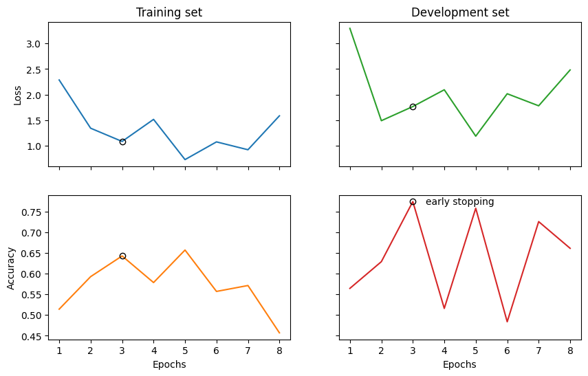
Results

Finally, we visualise the results and evaluate the model on the test data.

import matplotlib.pyplot as plt

fig, ((ax_tl, ax_tr), (ax_bl, ax_br)) = plt.subplots(2, 2, sharex=True, sharey='row', figsize=(10, 6))
ax_tl.set_title('Training set')
ax_tr.set_title('Development set')
ax_bl.set_xlabel('Epochs')
ax_br.set_xlabel('Epochs')
ax_bl.set_ylabel('Accuracy')
ax_tl.set_ylabel('Loss')

colours = iter(plt.rcParams['axes.prop_cycle'].by_key()['color'])
range_ = np.arange(1, len(trainer.train_epoch_costs)+1)
ax_tl.plot(range_, trainer.train_epoch_costs, color=next(colours))
ax_bl.plot(range_, trainer.train_eval_results['acc'], color=next(colours))
ax_tr.plot(range_, trainer.val_costs, color=next(colours))
ax_br.plot(range_, trainer.val_eval_results['acc'], color=next(colours))

# mark best model as circle
best_epoch = np.argmax(trainer.val_eval_results['acc'])
ax_tl.plot(best_epoch + 1, trainer.train_epoch_costs[best_epoch], 'o', color='black', fillstyle='none')
ax_tr.plot(best_epoch + 1, trainer.val_costs[best_epoch], 'o', color='black', fillstyle='none')
ax_bl.plot(best_epoch + 1, trainer.train_eval_results['acc'][best_epoch], 'o', color='black', fillstyle='none')
ax_br.plot(best_epoch + 1, trainer.val_eval_results['acc'][best_epoch], 'o', color='black', fillstyle='none')

ax_br.text(best_epoch + 1.4, trainer.val_eval_results['acc'][best_epoch], 'early stopping', va='center')

# print test accuracy
model.load(trainer.log_dir + '/best_model.lt')
val_acc = acc(model(val_circuits), val_labels)
print('Validation accuracy:', val_acc.item())

Validation accuracy: 0.7419354838709677

See also:

• Training: Classical case

• Training: Hybrid case

• Advanced: Manual training