Training: Classical case

In this section, we present a complete use case of lambeq’s training module, implementing a classical pipeline on the meaning classification dataset introduced in [Lea2021]. The goal is to classify simple sentences (such as “skillful programmer creates software” and “chef prepares delicious meal”) into two categories, food or IT. The dataset consists of 130 sentences created using a simple context-free grammar.

We will use a SpiderAnsatz to split large tensors into chains of smaller ones. The pipeline uses PyTorch as a backend.

Download code

Preparation

We start with importing PyTorch and specifying some training hyperparameters.

import torch

BATCH_SIZE = 30
EPOCHS = 30
LEARNING_RATE = 3e-2
SEED = 0

Input data

Let’s read the data and print some example sentences.

def read_data(filename):
    labels, sentences = [], []
    with open(filename) as f:
        for line in f:
            t = float(line[0])
            labels.append([t, 1-t])
            sentences.append(line[1:].strip())
    return labels, sentences


train_labels, train_data = read_data('../examples/datasets/mc_train_data.txt')
val_labels, val_data = read_data('../examples/datasets/mc_dev_data.txt')
test_labels, test_data = read_data('../examples/datasets/mc_test_data.txt')

train_data[:5]

['skillful man prepares sauce .',
 'skillful man bakes dinner .',
 'woman cooks tasty meal .',
 'man prepares meal .',
 'skillful woman debugs program .']

Targets are represented as 2-dimensional arrays:

train_labels[:5]

[[1.0, 0.0], [1.0, 0.0], [1.0, 0.0], [1.0, 0.0], [0.0, 1.0]]

Creating and parameterising diagrams

The first step is to convert sentences into string diagrams.

from lambeq import BobcatParser

parser = BobcatParser(verbose='text')

train_diagrams = parser.sentences2diagrams(train_data)
val_diagrams = parser.sentences2diagrams(val_data)
test_diagrams = parser.sentences2diagrams(test_data)

Tagging sentences.
Parsing tagged sentences.
Turning parse trees to diagrams.
Tagging sentences.
Parsing tagged sentences.
Turning parse trees to diagrams.
Tagging sentences.
Parsing tagged sentences.
Turning parse trees to diagrams.

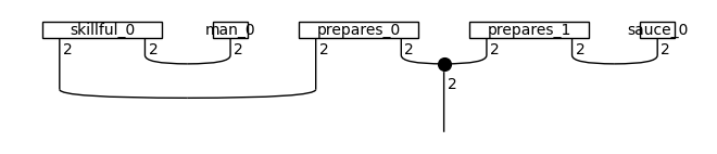
The produced diagrams need to be parameterised by a specific ansatz. For this experiment we will use a SpiderAnsatz.

from lambeq.backend.tensor import Dim

from lambeq import AtomicType, SpiderAnsatz

ansatz = SpiderAnsatz({AtomicType.NOUN: Dim(2),
                       AtomicType.SENTENCE: Dim(2)})

train_circuits = [ansatz(diagram) for diagram in train_diagrams]
val_circuits =  [ansatz(diagram) for diagram in val_diagrams]
test_circuits = [ansatz(diagram) for diagram in test_diagrams]

train_circuits[0].draw()

Training

Instantiate model

We can now initialise the model by importing the PytorchModel class, and passing all diagrams to the class method PytorchModel.from_diagrams().

from lambeq import PytorchModel

all_circuits = train_circuits + val_circuits + test_circuits
model = PytorchModel.from_diagrams(all_circuits)

Note

The model can also be instantiated by using the PytorchModel.from_checkpoint() method, if an existing checkpoint is available.

Additionally, the parameters can be initialised by invoking the PytorchModel.initialise_weights() method. Since Release 0.3.0, we initialise the parameters using a symmetric uniform distribution where the range is determined by the output dimension (flow codomain) of a box:

\[U\left(-\sqrt{3/\operatorname{dim}_{\text{flow_cod}}}, \sqrt{3/\operatorname{dim}_{\text{flow_cod}}}\right)\]

This ensures that the expected value of the L2 norm of the output of a box is approximately 1.

Define evaluation metric

Optionally, we can provide a dictionary of callable evaluation metrics with the signature metric(y_hat, y).

sig = torch.sigmoid

def accuracy(y_hat, y):
    return torch.sum(torch.eq(torch.round(sig(y_hat)), y))/len(y)/2  # half due to double-counting

eval_metrics = {"acc": accuracy}

Initialise trainer

Next step is to initialise a PytorchTrainer object. Because this is a binary classification task, we will use binary cross-entropy as the loss. As an optimizer, we choose Adam with weight decay.

Note

PytorchTrainer uses PyTorch’s native classes for optimisers and losses, instead of the lambeq equivalents.

from lambeq import PytorchTrainer

trainer = PytorchTrainer(
        model=model,
        loss_function=torch.nn.BCEWithLogitsLoss(),
        optimizer=torch.optim.AdamW,
        learning_rate=LEARNING_RATE,
        epochs=EPOCHS,
        evaluate_functions=eval_metrics,
        evaluate_on_train=True,
        verbose='text',
        seed=SEED)

Create datasets

To facilitate batching and data shuffling, lambeq provides a Dataset interface. Shuffling is enabled by default, and if not specified, the batch size is set to the length of the dataset. In our example we will use the BATCH_SIZE we have set above.

from lambeq import Dataset

train_dataset = Dataset(
            train_circuits,
            train_labels,
            batch_size=BATCH_SIZE)

val_dataset = Dataset(val_circuits, val_labels, shuffle=False)

Train

Now we can pass the datasets to the fit() method of the trainer to start the training.

trainer.fit(train_dataset, val_dataset, eval_interval=1, log_interval=5)

Epoch 5:   train/loss: 0.6518   valid/loss: 0.7119   train/acc: 0.5643   valid/acc: 0.5500
Epoch 10:  train/loss: 0.5804   valid/loss: 0.6197   train/acc: 0.5714   valid/acc: 0.6167
Epoch 15:  train/loss: 0.3311   valid/loss: 0.4577   train/acc: 0.8643   valid/acc: 0.7667
Epoch 20:  train/loss: 0.1054   valid/loss: 0.2346   train/acc: 0.9500   valid/acc: 0.9333
Epoch 25:  train/loss: 0.1346   valid/loss: 0.0438   train/acc: 0.9857   valid/acc: 1.0000
Epoch 30:  train/loss: 0.0005   valid/loss: 0.0283   train/acc: 0.9929   valid/acc: 1.0000

Training completed!

Note

The eval_interval controls the interval in which the model is evaluated on the validation dataset. Default is 1. If evaluation on the validation dataset is expensive, we recommend setting it to a higher value.

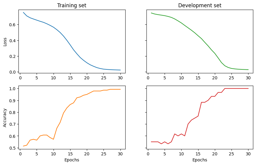
Results

Finally, we visualise the results and evaluate the model on the test data.

import matplotlib.pyplot as plt
import numpy as np

fig1, ((ax_tl, ax_tr), (ax_bl, ax_br)) = plt.subplots(2, 2, sharey='row', figsize=(10, 6))

ax_tl.set_title('Training set')
ax_tr.set_title('Development set')
ax_bl.set_xlabel('Epochs')
ax_br.set_xlabel('Epochs')
ax_bl.set_ylabel('Accuracy')
ax_tl.set_ylabel('Loss')

colours = iter(plt.rcParams['axes.prop_cycle'].by_key()['color'])
range_ = np.arange(1, trainer.epochs+1)
ax_tl.plot(range_, trainer.train_epoch_costs, color=next(colours))
ax_bl.plot(range_, trainer.train_eval_results['acc'], color=next(colours))
ax_tr.plot(range_, trainer.val_costs, color=next(colours))
ax_br.plot(range_, trainer.val_eval_results['acc'], color=next(colours))

# print test accuracy
test_acc = accuracy(model(test_circuits), torch.tensor(test_labels))
print('Test accuracy:', test_acc.item())

Test accuracy: 1.0

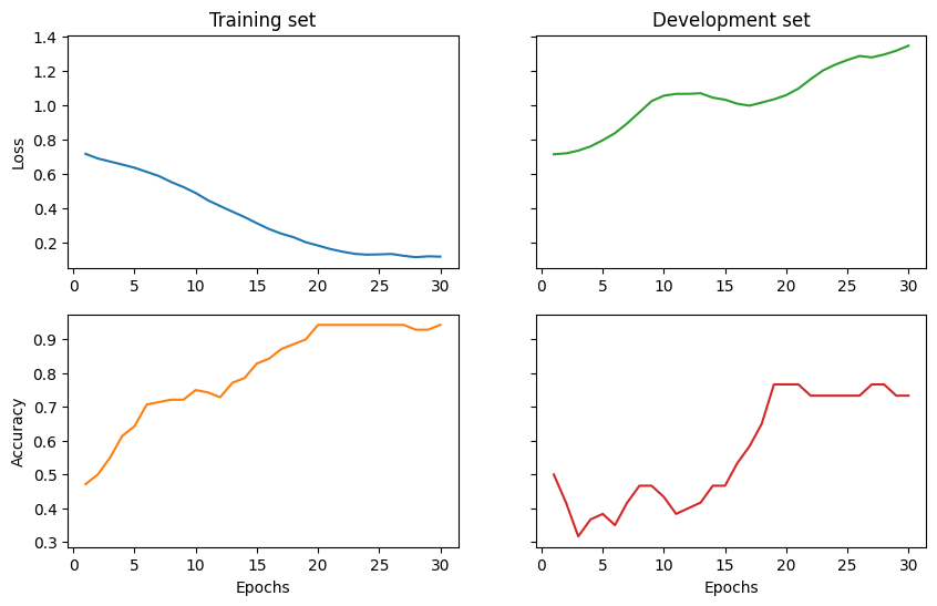
Adding custom layers to the model

In the default setting, the forward pass of a PytorchModel performs a simple tensor contraction of the tensorised diagrams. However, if one likes to add additional custom layers, one can create a custom model that inherits from PytorchModel and overwrite the PytorchModel.forward() method.

class MyCustomModel(PytorchModel):
    def __init__(self):
        super().__init__()
        self.net = torch.nn.Linear(2, 2)

    def forward(self, input):
        """define a custom forward pass here"""
        preds = self.get_diagram_output(input)
        preds = self.net(preds.float())
        return preds

The rest follows the same procedure as explained above, i.e. initialise a trainer, fit the model and visualise the results.

custom_model = MyCustomModel.from_diagrams(all_circuits)
custom_model_trainer = PytorchTrainer(
        model=custom_model,
        loss_function=torch.nn.BCEWithLogitsLoss(),
        optimizer=torch.optim.AdamW,
        learning_rate=LEARNING_RATE,
        epochs=EPOCHS,
        evaluate_functions=eval_metrics,
        evaluate_on_train=True,
        verbose='text',
        seed=SEED)

custom_model_trainer.fit(train_dataset, val_dataset, log_interval=5)

Epoch 5:   train/loss: 0.6729   valid/loss: 0.7965   train/acc: 0.6429   valid/acc: 0.3833
Epoch 10:  train/loss: 0.4602   valid/loss: 1.0563   train/acc: 0.7500   valid/acc: 0.4333
Epoch 15:  train/loss: 0.4580   valid/loss: 1.0329   train/acc: 0.8286   valid/acc: 0.4667
Epoch 20:  train/loss: 0.1645   valid/loss: 1.0594   train/acc: 0.9429   valid/acc: 0.7667
Epoch 25:  train/loss: 0.1098   valid/loss: 1.2642   train/acc: 0.9429   valid/acc: 0.7333
Epoch 30:  train/loss: 0.1957   valid/loss: 1.3476   train/acc: 0.9429   valid/acc: 0.7333

Training completed!

import matplotlib.pyplot as plt
import numpy as np

fig1, ((ax_tl, ax_tr), (ax_bl, ax_br)) = plt.subplots(2, 2, sharey='row', figsize=(10, 6))

ax_tl.set_title('Training set')
ax_tr.set_title('Development set')
ax_bl.set_xlabel('Epochs')
ax_br.set_xlabel('Epochs')
ax_bl.set_ylabel('Accuracy')
ax_tl.set_ylabel('Loss')

colours = iter(plt.rcParams['axes.prop_cycle'].by_key()['color'])
range_ = np.arange(1, trainer.epochs+1)
ax_tl.plot(range_, custom_model_trainer.train_epoch_costs, color=next(colours))
ax_bl.plot(range_, custom_model_trainer.train_eval_results['acc'], color=next(colours))
ax_tr.plot(range_, custom_model_trainer.val_costs, color=next(colours))
ax_br.plot(range_, custom_model_trainer.val_eval_results['acc'], color=next(colours))

# print test accuracy
test_acc = accuracy(model(test_circuits), torch.tensor(test_labels))
print('Test accuracy:', test_acc.item())

Test accuracy: 1.0

See also:

• Training: Hybrid case

• Training: Quantum case

• Advanced: Manual training