Training: Hybrid case
In this tutorial we train a pure quantum PennyLane model to solve a toy problem: classifying whether a given sentence is about cooking or computing. We also train a hybrid model that determines whether a given pair of sentences are talking about different topics.
We use an IQPAnsatz to convert string diagrams into quantum circuits. When passing these circuits to the PennyLaneModel, they are automatically converted into PennyLane circuits.
Preparation
We start by specifying some training hyperparameters and importing NumPy and PyTorch.
[1]:
BATCH_SIZE = 10
EPOCHS = 15
LEARNING_RATE = 0.1
SEED = 42
[2]:
import torch
import random
import numpy as np

torch.manual_seed(SEED)
random.seed(SEED)
np.random.seed(SEED)
Input data
Let’s read the data and print some example sentences.
[3]:
def read_data(filename):
    labels, sentences = [], []
    with open(filename) as f:
        for line in f:
            t = float(line[0])
            labels.append([t, 1-t])
            sentences.append(line[1:].strip())
    return labels, sentences


train_labels, train_data = read_data('../examples/datasets/mc_train_data.txt')
dev_labels, dev_data = read_data('../examples/datasets/mc_dev_data.txt')
test_labels, test_data = read_data('../examples/datasets/mc_test_data.txt')
[4]:
train_data[:5]
[4]:
['skillful man prepares sauce .',
 'skillful man bakes dinner .',
 'woman cooks tasty meal .',
 'man prepares meal .',
 'skillful woman debugs program .']
Targets are represented as 2-dimensional arrays:
[5]:
train_labels[:5]
[5]:
[[1.0, 0.0], [1.0, 0.0], [1.0, 0.0], [1.0, 0.0], [0.0, 1.0]]
Creating and parameterising diagrams
The first step is to convert the sentences into string diagrams.
[6]:
from lambeq import BobcatParser

reader = BobcatParser(verbose='text')

raw_train_diagrams = reader.sentences2diagrams(train_data)
raw_dev_diagrams = reader.sentences2diagrams(dev_data)
raw_test_diagrams = reader.sentences2diagrams(test_data)
Tagging sentences.
Parsing tagged sentences.
Turning parse trees to diagrams.
Tagging sentences.
Parsing tagged sentences.
Turning parse trees to diagrams.
Tagging sentences.
Parsing tagged sentences.
Turning parse trees to diagrams.
Simplify diagrams
We simplify the diagrams by removing cups with RemoveCupsRewriter; this reduces the number of post-selections in a diagram, allowing them to be evaluated more efficiently.
[7]:
from lambeq import RemoveCupsRewriter

remove_cups = RemoveCupsRewriter()

train_diagrams = [remove_cups(diagram) for diagram in raw_train_diagrams]
dev_diagrams = [remove_cups(diagram) for diagram in raw_dev_diagrams]
test_diagrams = [remove_cups(diagram) for diagram in raw_test_diagrams]
We can visualise these diagrams using draw().
[8]:
train_diagrams[0].draw()
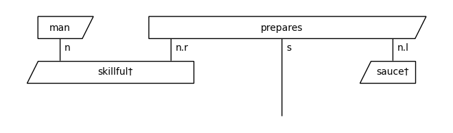
Create circuits
In order to run the experiments on a quantum computer, we apply a quantum ansatz to the string diagrams. For this experiment, we will use an IQPAnsatz, where noun wires (n) and sentence wires (s) are represented by one-qubit systems.
[9]:
from lambeq import AtomicType, IQPAnsatz

ansatz = IQPAnsatz({AtomicType.NOUN: 1, AtomicType.SENTENCE: 1},
                   n_layers=1, n_single_qubit_params=3)

train_circuits = [ansatz(diagram) for diagram in train_diagrams]
dev_circuits =  [ansatz(diagram) for diagram in dev_diagrams]
test_circuits = [ansatz(diagram) for diagram in test_diagrams]

train_circuits[0].draw(figsize=(6, 8))
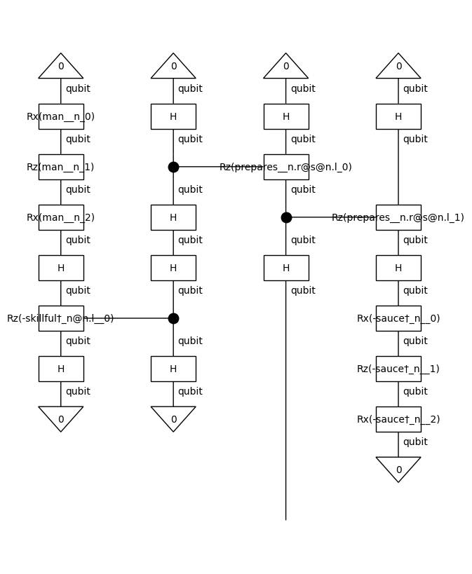
Training
Instantiate model
We instantiate a PennyLaneModel, by passing all diagrams to the class method PennyLaneModel.from_diagrams().
We also set probabilities=True so that the model outputs probabilities, rather than quantum states, which follows the behaviour of real quantum computers.
Furthermore, we set normalize=True so that the output probabilities sum to one. This helps to prevent passing very small values to any following layers in a hybrid model.
[10]:
from lambeq import PennyLaneModel

all_circuits = train_circuits + dev_circuits + test_circuits

# if no backend_config is provided, the default is used, which is the same as below
backend_config = {'backend': 'default.qubit'}  # this is the default PennyLane simulator
model = PennyLaneModel.from_diagrams(all_circuits,
                                     probabilities=True,
                                     normalize=True,
                                     backend_config=backend_config)
model.initialise_weights()
Running on a real quantum computer
We can choose to run the model on a real quantum computer, using Qiskit with IBMQ, or the Honeywell QAPI.
To use IBM devices we have to save our IBMQ API token to the PennyLane configuration file, as in the cell below.
[11]:
import pennylane as qml

qml.default_config['qiskit.ibmq.ibmqx_token'] = 'my_API_token'
qml.default_config.save(qml.default_config.path)
backend_config = {'backend': 'qiskit.ibmq',
                  'device': 'ibmq_manila',
                  'shots': 1000}
[12]:
q_model = PennyLaneModel.from_diagrams(all_circuits,
                                       probabilities=True,
                                       normalize=True,
                                       backend_config=backend_config)
q_model.initialise_weights()
To use Honeywell/Quantinuum devices we have to pass the email address of an account with access to the Honeywell/Quantinuum QAPI to the PennyLane configuration file.
The first time you run a circuit on a Honeywell device, you will be prompted to enter your password.
You can then run circuits without entering your password again for 30 days.
[13]:
qml.default_config['honeywell.global.user_email'] = ('my_Honeywell/Quantinuum_'
                                                     'account_email')
qml.default_config.save(qml.default_config.path)

backend_config = {'backend': 'honeywell.hqs',
                  'device': 'H1-1E',
                  'shots': 1000}
[14]:
h_model = PennyLaneModel.from_diagrams(all_circuits,
                                       probabilities=True,
                                       normalize=True,
                                       backend_config=backend_config)
h_model.initialise_weights()
Running these models on a real quantum computer takes a significant amount of time as the circuits must be sent to the backend and queued, so in the remainder of this tutorial we will use model, which uses the default PennyLane simulator, ‘default.qubit’.
Create datasets
To facilitate data shuffling and batching, lambeq provides a native Dataset class. Shuffling is enabled by default, and if not specified, the batch size is set to the length of the dataset.
[15]:
from lambeq import Dataset

train_dataset = Dataset(train_circuits,
                        train_labels,
                        batch_size=BATCH_SIZE)

val_dataset = Dataset(dev_circuits, dev_labels)
Training can either by done using the PytorchTrainer, or by using native PyTorch. We give examples of both in the following section.
Define loss and evaluation metric
When using PytorchTrainer we first define our evaluation metrics and loss function, which in this case will be the accuracy and the mean-squared error, respectively.
[16]:
def acc(y_hat, y):
    return (torch.argmax(y_hat, dim=1) ==
            torch.argmax(y, dim=1)).sum().item()/len(y)

def loss(y_hat, y):
    return torch.nn.functional.mse_loss(y_hat, y)
Initialise trainer
As PennyLane is compatible with PyTorch autograd, PytorchTrainer can automatically use many of the PyTorch optimizers, such as Adam to train our model.
[17]:
from lambeq import PytorchTrainer

trainer = PytorchTrainer(
    model=model,
    loss_function=loss,
    optimizer=torch.optim.Adam,
    learning_rate=LEARNING_RATE,
    epochs=EPOCHS,
    evaluate_functions={'acc': acc},
    evaluate_on_train=True,
    use_tensorboard=False,
    verbose='text',
    seed=SEED)
Train
We can now pass the datasets to the fit() method of the trainer to start the training.
[18]:
trainer.fit(train_dataset, val_dataset)
Epoch 1:   train/loss: 0.1207   valid/loss: 0.0919   train/acc: 0.7857   valid/acc: 0.8667
Epoch 2:   train/loss: 0.0486   valid/loss: 0.1035   train/acc: 0.9286   valid/acc: 0.9000
Epoch 3:   train/loss: 0.0364   valid/loss: 0.0621   train/acc: 0.9429   valid/acc: 0.9333
Epoch 4:   train/loss: 0.0466   valid/loss: 0.0392   train/acc: 0.9857   valid/acc: 1.0000
Epoch 5:   train/loss: 0.0120   valid/loss: 0.0126   train/acc: 0.9857   valid/acc: 1.0000
Epoch 6:   train/loss: 0.0014   valid/loss: 0.0178   train/acc: 1.0000   valid/acc: 1.0000
Epoch 7:   train/loss: 0.0022   valid/loss: 0.0079   train/acc: 1.0000   valid/acc: 1.0000
Epoch 8:   train/loss: 0.0041   valid/loss: 0.0061   train/acc: 1.0000   valid/acc: 1.0000
Epoch 9:   train/loss: 0.0003   valid/loss: 0.0108   train/acc: 1.0000   valid/acc: 1.0000
Epoch 10:  train/loss: 0.0001   valid/loss: 0.0205   train/acc: 1.0000   valid/acc: 0.9667
Epoch 11:  train/loss: 0.0001   valid/loss: 0.0281   train/acc: 1.0000   valid/acc: 0.9667
Epoch 12:  train/loss: 0.0005   valid/loss: 0.0309   train/acc: 1.0000   valid/acc: 0.9667
Epoch 13:  train/loss: 0.0004   valid/loss: 0.0314   train/acc: 1.0000   valid/acc: 0.9667
Epoch 14:  train/loss: 0.0004   valid/loss: 0.0308   train/acc: 1.0000   valid/acc: 0.9667
Epoch 15:  train/loss: 0.0011   valid/loss: 0.0286   train/acc: 1.0000   valid/acc: 0.9667

Training completed!
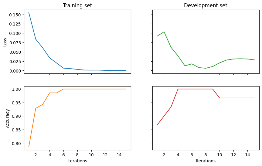
Results
Finally, we visualise the results and evaluate the model on the test data.
[19]:
import matplotlib.pyplot as plt

fig, ((ax_tl, ax_tr), (ax_bl, ax_br)) = plt.subplots(2, 2,
                                                     sharex=True,
                                                     sharey='row',
                                                     figsize=(10, 6))
ax_tl.set_title('Training set')
ax_tr.set_title('Development set')
ax_bl.set_xlabel('Iterations')
ax_br.set_xlabel('Iterations')
ax_bl.set_ylabel('Accuracy')
ax_tl.set_ylabel('Loss')

colours = iter(plt.rcParams['axes.prop_cycle'].by_key()['color'])
range_ = np.arange(1, trainer.epochs+1)
ax_tl.plot(range_, trainer.train_epoch_costs, color=next(colours))
ax_bl.plot(range_, trainer.train_eval_results['acc'], color=next(colours))
ax_tr.plot(range_, trainer.val_costs, color=next(colours))
ax_br.plot(range_, trainer.val_eval_results['acc'], color=next(colours))

# print test accuracy
pred = model(test_circuits)
labels = torch.tensor(test_labels)

print('Final test accuracy: {}'.format(acc(pred, labels)))
Final test accuracy: 0.9666666666666667
Using standard PyTorch
As we have a small dataset, we can use early stopping to prevent overfitting to the training data. In this case, we evaluate the performance of the model on the validation dataset every 5 epochs, and save a checkpoint if the validation accuracy has improved. If it does not improve for 10 epochs, we end the training, and load the model with the best validation accuracy.
[20]:
def accuracy(circs, labels):
    probs = model(circs)
    return (torch.argmax(probs, dim=1) ==
            torch.argmax(torch.tensor(labels), dim=1)).sum().item()/len(circs)
Training is the same as standard PyTorch. We initialize an optimizer, pass it the model parameters, and then run a training loop in which we compute the loss, run a backwards pass to compute the gradients, and then take an optimizer step.
[21]:
model = PennyLaneModel.from_diagrams(all_circuits)
model.initialise_weights()
optimizer = torch.optim.Adam(model.parameters(), lr=LEARNING_RATE)

best = {'acc': 0, 'epoch': 0}

for i in range(EPOCHS):
    epoch_loss = 0
    for circuits, labels in train_dataset:
        optimizer.zero_grad()
        probs = model(circuits)
        loss = torch.nn.functional.mse_loss(probs,
                                            torch.tensor(labels))
        epoch_loss += loss.item()
        loss.backward()
        optimizer.step()

    if i % 5 == 0:
        dev_acc = accuracy(dev_circuits, dev_labels)

        print('Epoch: {}'.format(i))
        print('Train loss: {}'.format(epoch_loss))
        print('Dev acc: {}'.format(dev_acc))

        if dev_acc > best['acc']:
            best['acc'] = dev_acc
            best['epoch'] = i
            model.save('model.lt')
        elif i - best['epoch'] >= 10:
            print('Early stopping')
            break

if best['acc'] > accuracy(dev_circuits, dev_labels):
    model.load('model.lt')
Epoch: 0
Train loss: 1.8359988629817963
Dev acc: 0.5333333333333333
Epoch: 5
Train loss: 0.19099989160895348
Dev acc: 0.9
Epoch: 10
Train loss: 0.059448788000736386
Dev acc: 0.9666666666666667
Evaluate test accuracy
[22]:
print('Final test accuracy: {}'.format(accuracy(test_circuits, test_labels)))
Final test accuracy: 0.9
Hybrid models
This model determines whether a pair of diagrams are about the same or different topics.
It does this by first running the pair circuits to get a probability output for each, and then concatenating them together and passing them to a simple neural network.
We expect the circuits to learn to output [0, 1] or [1, 0] depending on the topic they are referring to (cooking or computing), and the neural network to learn the XOR function to determine whether the topics are the same (output 0) or different (output 1).
PennyLane allows us to train both the circuits and the NN simultaneously using PyTorch autograd.
[23]:
BATCH_SIZE = 50
EPOCHS = 100
LEARNING_RATE = 0.1
SEED = 2
As the probability outputs from our circuits are guaranteed to be positive, we transform these outputs x by 2 * (x - 0.5), giving inputs to the neural network in the range [-1, 1].
This helps us to avoid “dying ReLUs”, which could otherwise occur if all the input weights to a given hidden neuron were negative; in this case, the overall input to the neuron would be negative, and ReLU would set the output of it to 0, leading to the gradient of all these weights being 0 for all samples, causing the neuron to never learn.
(A couple of alternative approaches could also involve initialising all the neural network weights to be positive, or using LeakyReLU as the activation function).
[24]:
from torch import nn

class XORSentenceModel(PennyLaneModel):
    def __init__(self, **kwargs):
        PennyLaneModel.__init__(self, **kwargs)

        self.xor_net = nn.Sequential(nn.Linear(4, 10),
                                     nn.ReLU(),
                                     nn.Linear(10, 1),
                                     nn.Sigmoid())

    def forward(self, diagram_pairs):
        first_d, second_d = zip(*diagram_pairs)
        evaluated_pairs = torch.cat((self.get_diagram_output(first_d),
                                     self.get_diagram_output(second_d)),
                                    dim=1)
        evaluated_pairs = 2 * (evaluated_pairs - 0.5)
        return self.xor_net(evaluated_pairs)
Make paired dataset
Our model is going to determine whether a given pair of sentences are talking about different topics, so we need to construct a dataset of pairs of diagrams for the train, dev, and test data.
[25]:
from itertools import combinations

def make_pair_data(diagrams, labels):
    pair_diags = list(combinations(diagrams, 2))
    pair_labels = [int(x[0] == y[0]) for x, y in combinations(labels, 2)]
    return pair_diags, pair_labels

train_pair_circuits, train_pair_labels = make_pair_data(train_circuits,
                                                        train_labels)
dev_pair_circuits, dev_pair_labels = make_pair_data(dev_circuits,
                                                    dev_labels)
test_pair_circuits, test_pair_labels = make_pair_data(test_circuits,
                                                      test_labels)
There are lots of pairs (2415 train pairs), so we’ll sample a subset to make this example train more quickly.
[26]:
TRAIN_SAMPLES, DEV_SAMPLES, TEST_SAMPLES = 300, 200, 200
[27]:
train_pair_circuits, train_pair_labels = (
    zip(*random.sample(list(zip(train_pair_circuits, train_pair_labels)),
                       TRAIN_SAMPLES)))
dev_pair_circuits, dev_pair_labels = (
    zip(*random.sample(list(zip(dev_pair_circuits, dev_pair_labels)), DEV_SAMPLES)))
test_pair_circuits, test_pair_labels = (
    zip(*random.sample(list(zip(test_pair_circuits, test_pair_labels)), TEST_SAMPLES)))
Initialise model
As XORSentenceModel inherits from PennyLaneModel, we can again pass in probabilities=True and normalize=True to from_diagrams().
[28]:
all_pair_circuits = (train_pair_circuits +
                     dev_pair_circuits +
                     test_pair_circuits)
a, b = zip(*all_pair_circuits)

model = XORSentenceModel.from_diagrams(a + b)
model.initialise_weights()
model = model

train_pair_dataset = Dataset(train_pair_circuits,
                             train_pair_labels,
                             batch_size=BATCH_SIZE)

optimizer = torch.optim.Adam(model.parameters(), lr=LEARNING_RATE)
Train and log accuracies
We train the model using pure PyTorch in the exact same way as above.
[29]:
def accuracy(circs, labels):
    predicted = model(circs)
    return (torch.round(torch.flatten(predicted)) ==
            torch.Tensor(labels)).sum().item()/len(circs)
[30]:
best = {'acc': 0, 'epoch': 0}

for i in range(EPOCHS):
    epoch_loss = 0
    for circuits, labels in train_pair_dataset:
        optimizer.zero_grad()
        predicted = model(circuits)
        loss = torch.nn.functional.binary_cross_entropy(
            torch.flatten(predicted), torch.Tensor(labels))
        epoch_loss += loss.item()
        loss.backward()
        optimizer.step()

    if i % 5 == 0:
        dev_acc = accuracy(dev_pair_circuits, dev_pair_labels)

        print('Epoch: {}'.format(i))
        print('Train loss: {}'.format(epoch_loss))
        print('Dev acc: {}'.format(dev_acc))

        if dev_acc > best['acc']:
            best['acc'] = dev_acc
            best['epoch'] = i
            model.save('xor_model.lt')
        elif i - best['epoch'] >= 10:
            print('Early stopping')
            break

if best['acc'] > accuracy(dev_pair_circuits, dev_pair_labels):
    model.load('xor_model.lt')
    model = model
Epoch: 0
Train loss: 4.2918784618377686
Dev acc: 0.53
Epoch: 5
Train loss: 3.722463011741638
Dev acc: 0.54
Epoch: 10
Train loss: 0.5063610002398491
Dev acc: 0.9
Epoch: 15
Train loss: 5.019097626209259
Dev acc: 0.56
Epoch: 20
Train loss: 2.7006355822086334
Dev acc: 0.6
Early stopping
[31]:
print('Final test accuracy: {}'.format(accuracy(test_pair_circuits,
                                                test_pair_labels)))
Final test accuracy: 0.95
Analysing the internal representations of the model
We hypothesised that the quantum circuits would be able to separate the representations of sentences about food and cooking, and that the classical NN would learn to XOR these representations to give the model output. Here we can look at parts of the model separately to determine whether this hypothesis was accurate.
First, we can look at the output of the NN when given the 4 possible binary inputs to XOR.
[32]:
xor_labels = [[1, 0, 1, 0], [0, 1, 0, 1], [1, 0, 0, 1], [0, 1, 1, 0]]
# the first two entries correspond to the same label for both sentences, the last two to different labels
xor_tensors = torch.tensor(xor_labels).float()

model.xor_net(xor_tensors).detach().numpy()
[32]:
array([[0.9858948 ],
       [0.91964245],
       [0.03415415],
       [0.15316254]], dtype=float32)
We can see that in the case that the labels are the same, the outputs are significantly greater than 0.5, and in the case that the labels are different, the outputs are significantly less than 0.5, and so the NN seems to have learned the XOR function.
We can also look at the outputs of some of the test circuits to determine whether they have been able to seperate the two classes of sentences.
[33]:
FOOD_IDX, IT_IDX = 0, 6
symbol_weight_map = dict(zip(model.symbols, model.weights))
[34]:
print(test_data[FOOD_IDX])

p_circ = test_circuits[FOOD_IDX].to_pennylane(probabilities=True)
p_circ.initialise_concrete_params(symbol_weight_map)
unnorm = p_circ.eval().detach().numpy()

unnorm / np.sum(unnorm)
woman prepares tasty dinner .
[34]:
array([0.3952476 , 0.60475236], dtype=float32)
[35]:
print(test_data[IT_IDX])

p_circ = test_circuits[IT_IDX].to_pennylane(probabilities=True)
p_circ.initialise_concrete_params(symbol_weight_map)
unnorm = p_circ.eval().detach().numpy()

unnorm / np.sum(unnorm)
skillful person runs software .
[35]:
array([0.92366177, 0.07633827], dtype=float32)
From these examples, it seems that the circuits are able to strongly differentiate between the two topics, assigning approximately [0, 1] to the sentence about food, and [1, 0] to the sentence about computing.
See also: