A complete use case

In this section we present a complete use case of manual training (without using the training package), based on the meaning classification dataset introduced in [Lea2021]. The goal is to classify simple sentences (such as “skillful programmer creates software” and “chef prepares delicious meal”) into two categories, food or IT. The dataset consists of 130 sentences created using a simple context-free grammar.

We will use a SpiderAnsatz to split large tensors into chains of smaller ones. For differentiation we will use JAX, and we will apply simple gradient-descent optimisation to train the tensors.

Download code

Preparation

We start with a few essential imports.

import warnings
warnings.filterwarnings('ignore')  # Ignore warnings

from discopy.tensor import Tensor
from jax import numpy as np
import numpy

np.random = numpy.random
Tensor.np = np

np.random.seed(123458)  # Fix the seed

Note

Note the Tensor.np = np assignment in the above code. This is required in older versions of DisCoPy to let it know that from now on we use JAX’s version of numpy.

Let’s read the datasets:

Input data

# Read data
def read_data(fname):
    with open(fname, 'r') as f:
        lines = f.readlines()
    data, targets = [], []
    for ln in lines:
        t = int(ln[0])
        data.append(ln[1:].strip())
        targets.append(np.array([t, not(t)], dtype=np.float32))
    return data, np.array(targets)

train_data, train_targets = read_data('../examples/datasets/mc_train_data.txt')
test_data, test_targets = read_data('../examples/datasets/mc_test_data.txt')

WARNING:absl:No GPU/TPU found, falling back to CPU. (Set TF_CPP_MIN_LOG_LEVEL=0 and rerun for more info.)

The first few lines of the train dataset:

train_data[:10]

['skillful man prepares sauce .',
 'skillful man bakes dinner .',
 'woman cooks tasty meal .',
 'man prepares meal .',
 'skillful woman debugs program .',
 'woman prepares tasty meal .',
 'person runs program .',
 'person runs useful application .',
 'woman prepares sauce .',
 'woman prepares dinner .']

Targets are represented as 2-dimensional arrays:

train_targets

DeviceArray([[1., 0.],
             [1., 0.],
             [1., 0.],
             ...,
             [0., 1.],
             [1., 0.],
             [0., 1.]], dtype=float32)

Creating and parameterising diagrams

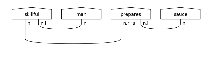
First step is to convert sentences into string diagrams:

# Parse sentences to diagrams

from lambeq import BobcatParser

parser = BobcatParser(verbose='suppress')
train_diagrams = parser.sentences2diagrams(train_data)
test_diagrams = parser.sentences2diagrams(test_data)

train_diagrams[0].draw(figsize=(8,4), fontsize=13)

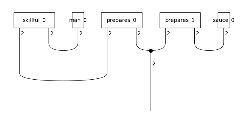
The produced diagrams need to be parameterised by a specific ansatz. For this experiment we will use a SpiderAnsatz.

# Create ansatz and convert to tensor diagrams

from lambeq import AtomicType, SpiderAnsatz
from discopy import Dim

N = AtomicType.NOUN
S = AtomicType.SENTENCE

# Create an ansatz by assigning 2 dimensions to both
# noun and sentence spaces
ansatz = SpiderAnsatz({N: Dim(2), S: Dim(2)})

train_circuits = [ansatz(d) for d in train_diagrams]
test_circuits = [ansatz(d) for d in test_diagrams]

all_circuits = train_circuits + test_circuits

all_circuits[0].draw(figsize=(8,4), fontsize=13)

Creating a vocabulary

We are now ready to create a vocabulary.

# Create vocabulary

from sympy import default_sort_key

vocab = sorted(
   {sym for circ in all_circuits for sym in circ.free_symbols},
    key=default_sort_key
)
tensors = [np.random.rand(w.size) for w in vocab]

tensors[0]

array([0.17825215, 0.02690565])

Training

Define loss function

This is a binary classification task, so we will use binary cross entropy as the loss.

def sigmoid(x):
    return 1 / (1 + np.exp(-x))

def loss(tensors):
    # Lambdify
    np_circuits = [c.lambdify(*vocab)(*tensors) for c in train_circuits]
    # Compute predictions
    predictions =  sigmoid(np.array([c.eval().array for c in np_circuits]))

    # binary cross-entropy loss
    cost = -np.sum(train_targets * np.log2(predictions)) / len(train_targets)
    return cost

The loss function follows the steps below:

1. The symbols in the training diagrams are replaced with concrete numpy arrays.

2. The resulting tensor networks are evaluated and produce results.

3. Based on the predictions, an average loss is computed for the specific iteration.

We use JAX in order to get a gradient function on the loss, and “just-in-time” compile it to improve speed:

from jax import jit, grad

training_loss = jit(loss)
gradient = jit(grad(loss))

Train

We are now ready to start training. The following loop computes gradients and uses them to update the tensors associated with the symbols.

training_losses = []

epochs = 90

for i in range(epochs):

    gr = gradient(tensors)
    for k in range(len(tensors)):
        tensors[k] = tensors[k] - gr[k] * 1.0

    training_losses.append(float(training_loss(tensors)))

    if (i + 1) % 10 == 0:
        print(f"Epoch {i + 1} - loss {training_losses[-1]}")

Epoch 10 - loss 0.18159326910972595
Epoch 20 - loss 0.028411218896508217
Epoch 30 - loss 0.014218389056622982
Epoch 40 - loss 0.009306452237069607
Epoch 50 - loss 0.006690497510135174
Epoch 60 - loss 0.0050796098075807095
Epoch 70 - loss 0.004009702242910862
Epoch 80 - loss 0.003261777339503169
Epoch 90 - loss 0.0027179380413144827

Evaluate

Finally, we use the trained model on the test dataset:

# Testing

np_test_circuits = [c.lambdify(*vocab)(*tensors) for c in test_circuits]
test_predictions =  sigmoid(np.array([c.eval().array for c in np_test_circuits]))

hits = 0
for i in range(len(np_test_circuits)):
    target = test_targets[i]
    pred = test_predictions[i]
    if np.argmax(target) == np.argmax(pred):
        hits += 1

print("Accuracy on test set:", hits / len(np_test_circuits))

Accuracy on test set: 0.9

Working with quantum circuits

The process when working with quantum circuits is very similar, with two important differences:

1. The parameterisable part of the circuit is an array of parameters, as described in Section Circuit Symbols, instead of tensors associated to words.

2. If optimisation takes place on quantum hardware, standard automatic differentiation cannot be used. An alternative is to use a gradient-approximation technique, such as Simultaneous Perturbation Stochastic Approximation (SPSA).

More information can be also found in [Mea2020] and [Lea2021], the papers that describe the first NLP experiments on quantum hardware.

See also:

• Classical pipeline with Pytorch

• Quantum pipeline with tket

• Quantum pipeline with JAX